A Deep Dive into How Flexibility Affects The Bias and Variance Trade Off

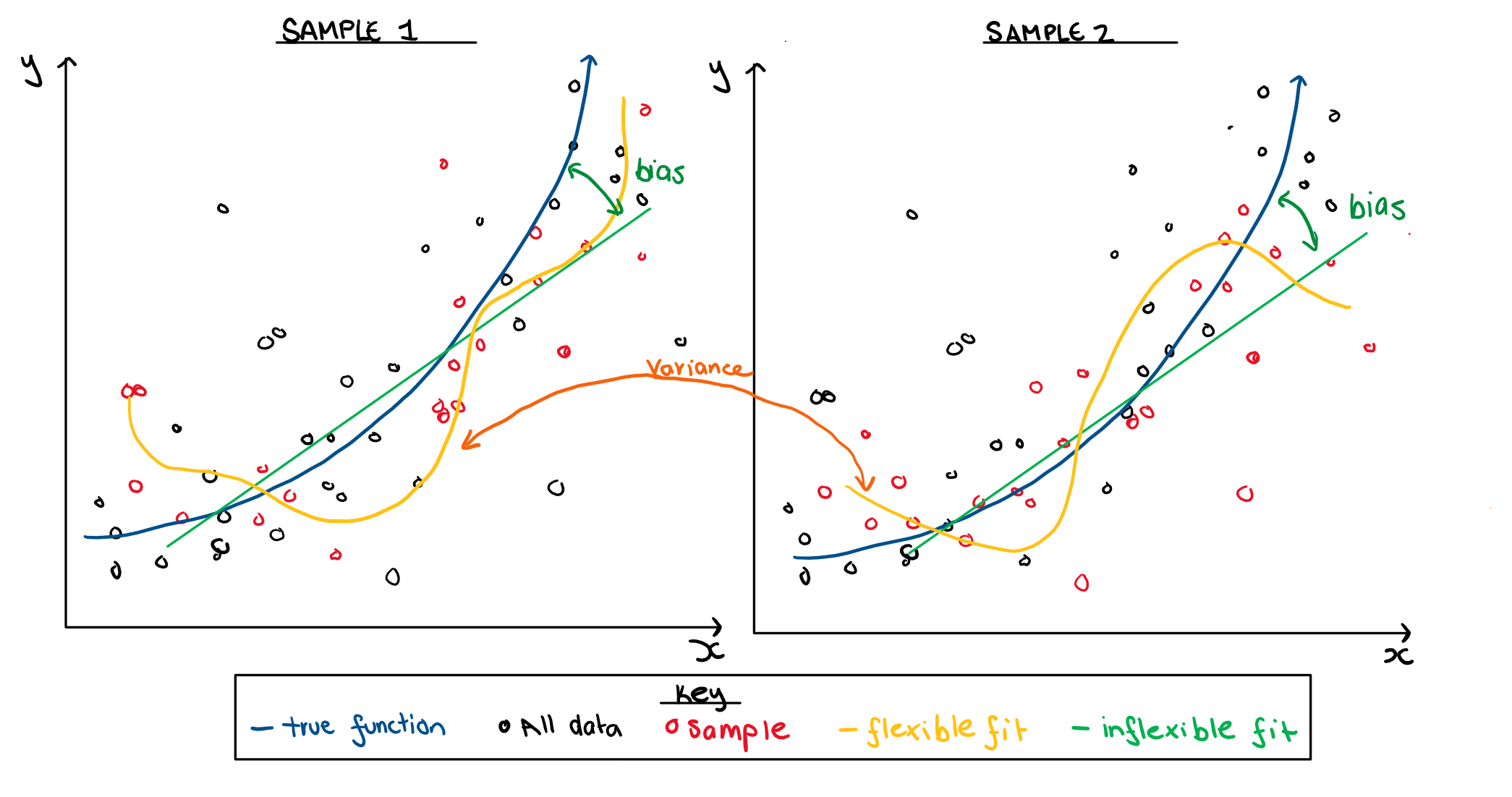
When we are building a machine learning model you have a choice of a simple, which would be an inflexible, model vs a complicated, or very flexible model. We need to decide how flexible the model should be to work well for future samples. An inflexible model may not reflect a complex underlying process adequately and hence would be biased. A flexible model has the capacity to capture a complex underlying process but the fitted version might change from one sample to another enormously, which is called variance. This difference is illustrated in the figure below.

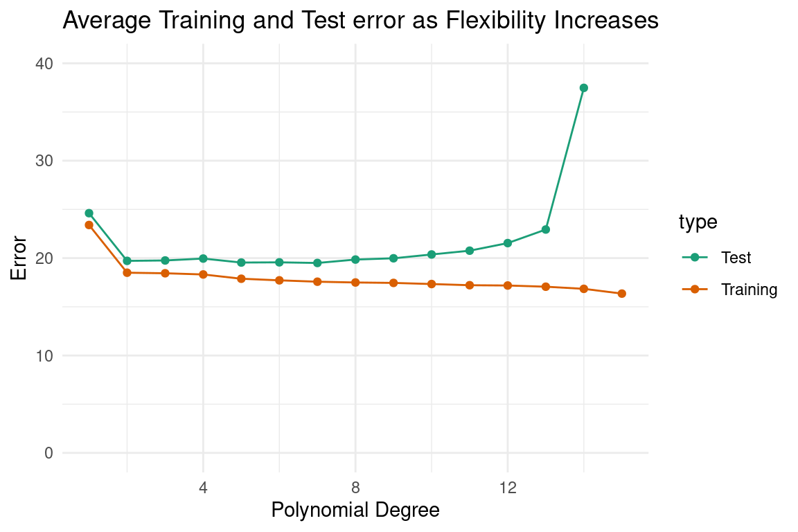
When we think of how the bias and variance change with flexibility, we typically only look at its behaviour on average. In the plot below, the left side corresponds to an inflexible model and the right side corresponds to a flexible model. We can see that the test error stay slightly above the training as flexibility increases, until the text error shoots up. Visualisations like this are shown frequently in the textbook “An Introduction to Statistical Learning with Applications in R” by Gareth James, Daniela Witten, Trevor Hastie and Robert Tibshirani, which largely inspired this blog post. While this explains the behaviour of our test error on average, it doesn’t give a complete understanding of how our test error estimate will act within any individual sample. This is where we find the benefit of understanding the error distribution. The distribution of the test error allows us to not only understand the average behaviour, but also how that behaviour may change from sample to sample.

Flexibility’s Influence on Test Error

When changing the flexibility of a model, the test error distribution will go through three phases, that affect both its expected value, and variance.

Phase 1: Decreasing Bias in Model

When our model is biased, we are forcing our data into constraints that don’t reflect the true relationship between the variables. Since we have not captured the true relationship of the parameters, any sample drawn from our population will also have a more complicated relationship than that of our model, and have error from bias. This relationship is illustrated below, where our high error is largely the result of too much bias in the model. Both distributions are similar to each other, but far from zero.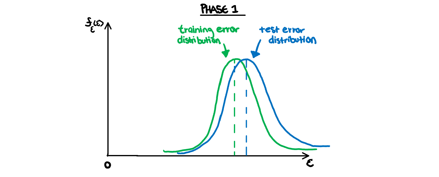

Phase 2: Optimal Fit

Increasing the flexibility will reduce the bias which will decrease the error. The optimal error will have smaller error for both training and test, but they will both be pretty similar. If you have captured the true relationship of the data with your model (if there is one), the distributions should perfectly overlap. This is unlikely to happen, since your model will always have a bias towards any quirks in your training set, and thus perform better on that set most of the time. So we instead will interpret the optimal fit is when the test error reaches its minimum (before the variance causes the total error to start to increase).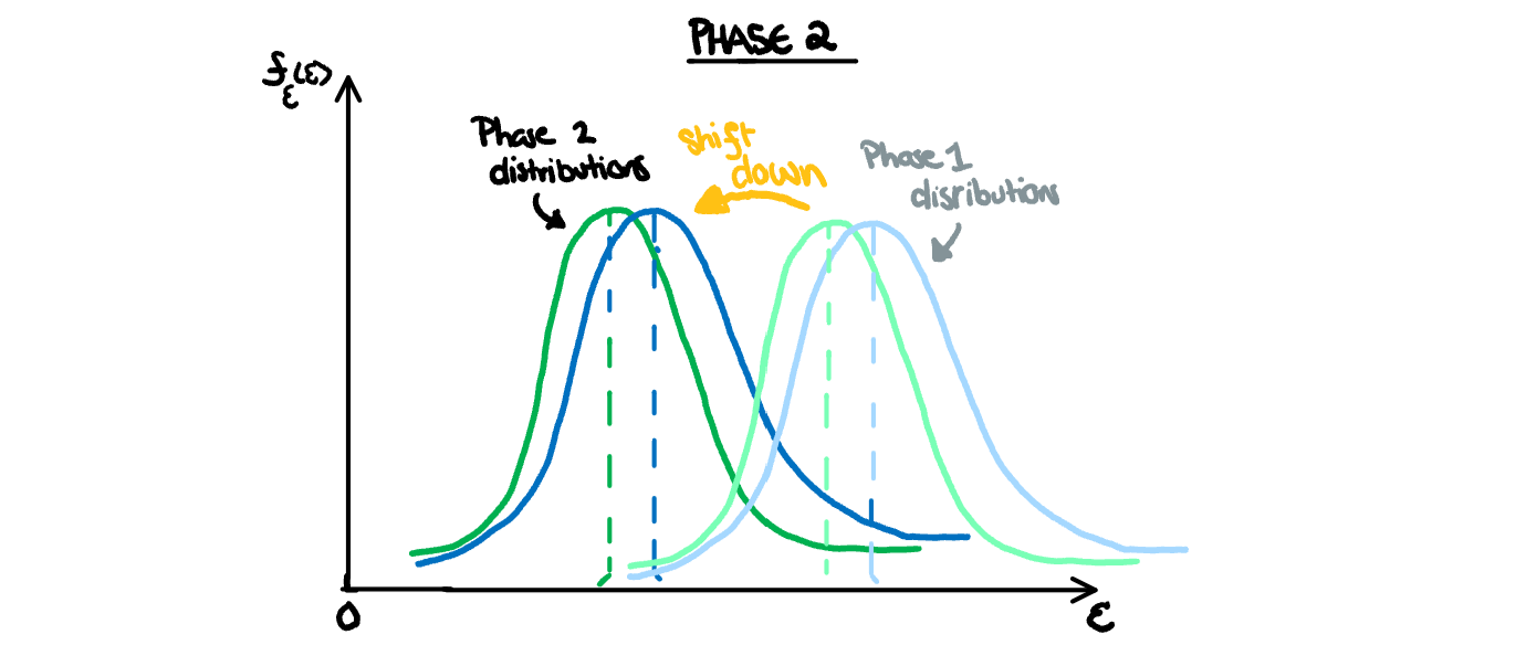

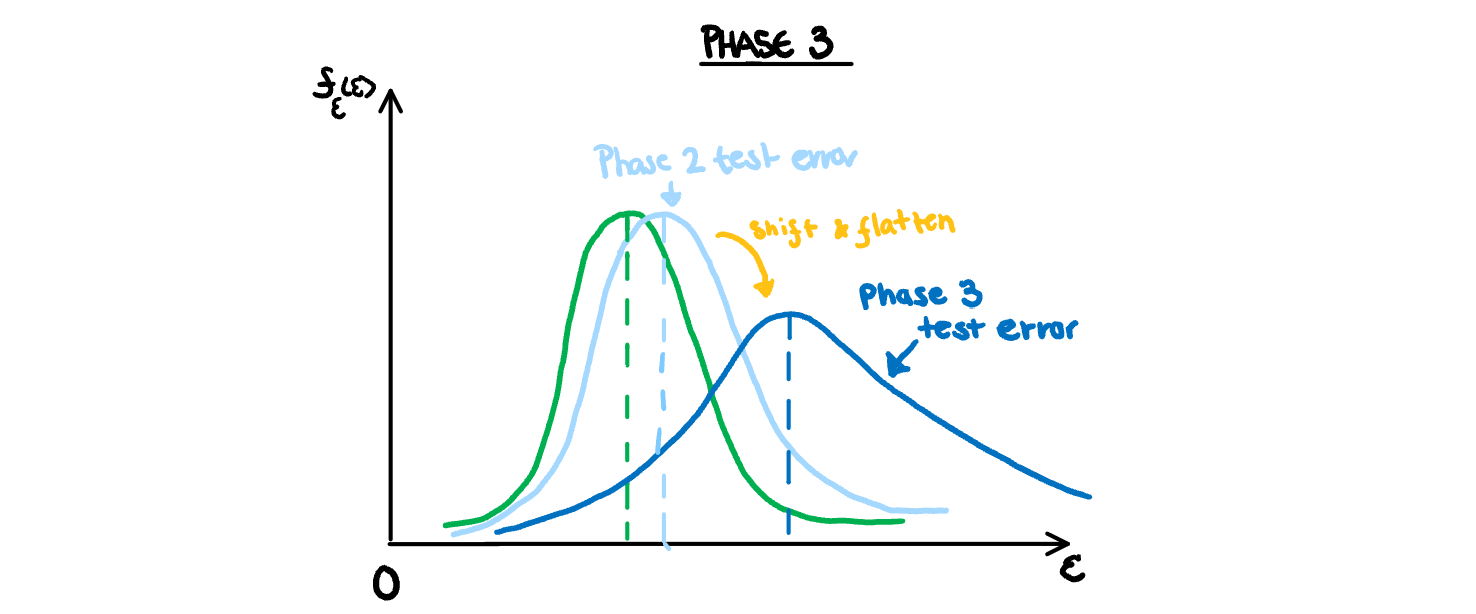
Phase 3: Increasing Variance in Model

As we start to overfit our model, we introduce more error from variance than we are losing from decreasing bias. This has two effects on the distribution of the estimated test error. First, it causes the distribution to shift upwards as we have once again missed the true relationship in the population. This miss is different from bias however, as we have overfit our model to the specifics of the test set sample, thus new samples drawn from the same population will not have a similar error. This causes the distributions to shift away from each other. Additionally, the variance of the test error estimate will also increase. Overfitting means a higher penalty for samples that just happen to be different from our training set, and a higher reward for those that just happen to have similar quirks. Ultimately that makes the estimates more unreliable, and thus have a higher variance.

Understanding with an Example

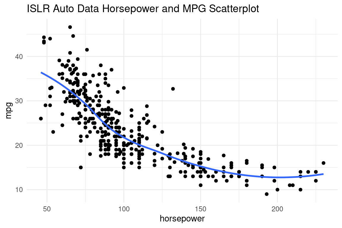
This influence from flexibility can best be seen with an example. To illustrate this, we will use the Auto data from the ISLR package, and fit a model to predict mpg using a polynomial of horsepower. If we take a look at the scatterplot of the two variables below, we can see that the linear model might not be flexible enough, but anything more flexible than a polynomial of about 4, will very likely overfit to the training sample. The plot below shows the data with a loess fit.

We can see the effect on the distributions using the animated density plot below. Here we have taken 100 different samples, and fit a model that predicts mpg using a polynomial degree of 1 to 15 of horsepower. Here we can see the above hand drawn illustration and interpretation of the variable relationship play out. Initially, increasing the flexibility of our model eliminates bias and causes both distributions to shift down. At polynomial degree 4, they stop at the minimum, and then for polynomial degrees higher than that, variance is introduced, and the test error increases in both expected value and variance.

png

Sample to Sample Changes

Here it is important to highlight the difference between a population and a sample, so we can better understand how an unfortunate test and training split can hurt error estimates. A population is all the data on what you are trying to make an inference on. For example, if I want to make an inference on the true relationship between mpg and horsepower, the Auto data is a sample of that. Generally we would be interested to make statements for mgp and horsepower for all possible cars, where all possible cars would be our population. If I want to make an inference on the relationship between mpg and horsepower in the Auto dataset (which is a weirdly specific realm to keep your inferences to but each to his own I guess) then this data is the population sample. For our sample to be representative, it needs to both be randomly drawn, and large enough. Unfortunately, even when we draw our samples to be decently large in size, and random, we will still occasionally get some unrepresentative splits. A sample that is unlike the population will bring the validity of any inference we try to make using that sample (including predictive models) into disrepute. Below is an illustration on how the sample will influence the fit among other interpretations.

png

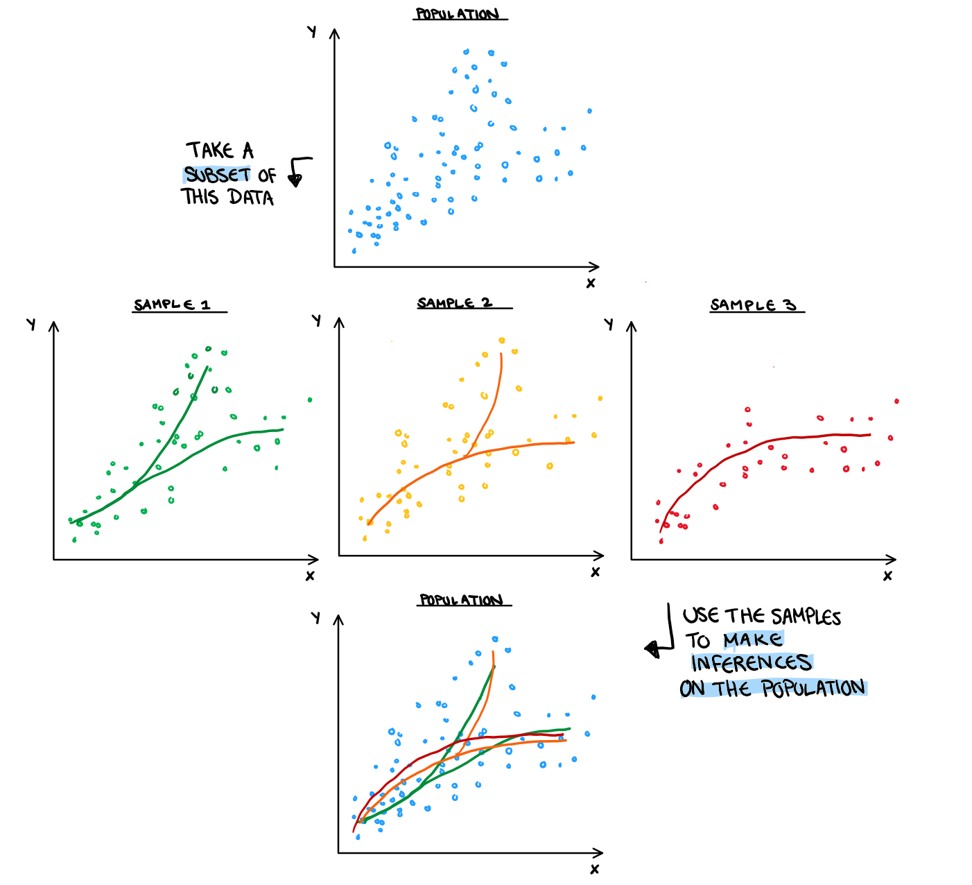
That being said, it’s highly unlikely to get a difference that dramatic in an actual sample. In reality, minor, almost invisible to the eye differences in your sample will create large differences in your MSE estimates.

An Example of Sample Influence on Error

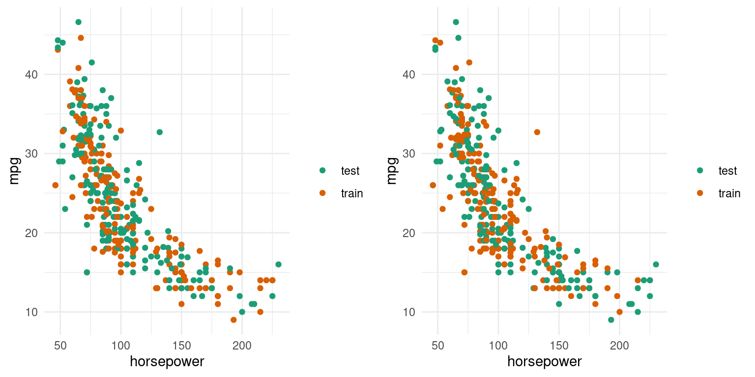
The scatterplots below shows two of the training and test sample splits that were used in the phases example. One produced the best test error on the polynomial 15 model (MSE= 105) and the other, the worst (MSE=9837). Is there a remarkable difference?

How Our Estimation Method Influences Our Test Error Distribution

A glaring issue with our test error estimate is its high variance, which means less certainty in the conclusions we draw from our test estimates. If we want a test error estimation method that is less susceptible to this issue of variance, we could try using a cross validation method. All methods, like the test error shown above, will still follow the general phases caused by increasing flexibility, but some have a lower overall variance (at the cost of more bias).

The Phases Example Using Cross Validation

When we originally looked at the test error, it was estimated with the validation set approach (test in the plot) for simplicity. Now, let’s redo those distribution estimations of error from the mpg and horsepower models, but also look at the distribution of the 10-fold (k10cv), and 5-fold cross (k5cv) validation methods.

png

Here we can see the bias variance trade off play out with our estimates of test error, just as they would with our model fit. Our cross-validation methods in order of increasing variance are:

5-fold CV < 10-fold CV < Validation Set Method

The methods in order of increasing bias are:

10-fold CV < 5-fold CV < Validation Set Method

In general, the k-fold CV bias and variance depends on the value of k, where LOOCV (k=n) is approximately unbiased.

To Summarise…

As the flexibility of our model increases, we know that the estimated model will have a decrease in bias and increase in variance. This change in our model causes both a change in the mean and variance of our estimated test error. A lot of the difference is caused by the increasing impact of our random sample split, however it is not something that is visually noticeable. Like the model, the method of test error estimation also has its own bias and variance trade off, and it can be balanced using cross validation methods.

This work is licensed under a Creative Commons Attribution-NonCommercial-ShareAlike 4.0 International License.